NLP-ALL YOU NEED TO KNOW

What is Natural Language Processing?

A language is a way we humans communicate with each other. Each day we produce data from Emails, SMS, Tweets, etc. We must have methods to understand this type of data, just like we do for other types of data. We will learn some of the basic and important techniques in Natural Language Processing.
Natural-Language Process (NLP) is a neighborhood of applied science and computer science concerned with the interactions between computers and human (natural) languages, specifically how to program computers to productively method giant amounts of natural language data.
In straightforward terms, natural language process (NLP) is that the ability of computers to know human speech because it is spoken. NLP helps to investigate, understand, and derive which means from human language in the form of good and helpful manner.
It is the branch of Data Science that deals with explanation worthy information by analyzing, understanding, and utilizing context from the text data. It builds interactions between machines and natural languages by planning and building applications.
Why Natural Language Processing(NLP )?

Natural+ Language+ Processing= Way of making our machine understands our human language in form of text/speech etc. And extract useful services from it.
Data can be form of many formats like audio, video, text, tables, images etc. In order to deal with text and speech/audio kind of data for extracting information we apply NLP.
NLP provides various tools and techniques to deal with text data specifically.
Why NLP has taken its pace now-a-days?
1) As day to day, data usage increased which led to different formats of data.
2) Data veracity, variety, volume made NLP to come into its limelight and the case studies or the applications of NLP are irreplaceable.
How to perform Natural Language Processing (NLP)?
The answer would be text pre-processing and text feature engineering. As everything in the world would be quantified, the same sense works on text data.
The process of extracting information about the text data with the corresponding steps for numeric conversion or quantifying or analytical purposes is called Text Pre-processing.
It is the prominent step that one has to be done for feature extraction and to perform Exploratory Data Analysis by word cloud, constructing histogram by word frequency correlation over topics or documents etc.
Any data to make it compatible with machine, has to undergo few pre-processing steps followed by text cleaning.
- Text Cleaning
Before cleaning the text, we should know about text noise.
Text Noise
It is unwanted or useless information present in text data. It is caused due to reasons such as Human errors, Data entry errors, Less accurate digitization software, Less accurate machine translation, Web scraping
Common Entities (Stop words, URLs, hashtags, punctuations, numbers),Slangs (words which are absent in the dictionaries), Spelling and Grammar errors, keyword Variations are the examples of text noise.
Text cleaning is very important because it reduce the dimensions of data, simples machine learning models, gets rid of repetitive information and focuses on useful entities and information. Text Cleaning is the process of removal of text noise as follows:
•Fix the decoding of text: Text data obtained from web is often present in a different encoding. So, it must be converted into a standard encoding : utf8
•Escaping HTML Characters: Examples such as < > & must be removed by using Regular Expressions, List iteration, appropriate libraries.
•Apostrophe Lookup: It is the variations with the words. For example: it’s -> it is or it has. We need to solve using Regular expressions or lookup table.
•Removal of stop words: We need to remove commonly used words : “a”, “an”, “the”, “is”, “am”, “are”, “of” etc. by using appropriate libraries, list iteration as they are less informative about the context.
•Noisy Entities: Removal noisy entities such as URLs, Hashtag words, Mention Words using regular expressions.
•Punctuations: Remove all symbols like emoticons, regular punctuations, connectors. For example: From (I, went to United States !!) to I went to United States.
•Keyword Normalization: Normalization is the process of converting a token into its base form (morpheme). It helps in reducing data dimensionality, text cleaning. Stemming and Lemmatization are the types of normalization.
•Morpheme : It is the base form of a word. Structure of token : <prefix> <morpheme> <suffix>. Example : Antisocialist : Anti +social + ist
•Stemming: Stemming converts tokens to base form without looking into grammar and POS tagging. For example: Words like “laughing”, “laughed”, “laughs”, “laugh” are converted into “laugh” and scientist name Fleming to Flem.
The disadvantage of stemming would be it may generate non-meaningful terms like his teams are not winning to hi team are not winn.
•Lemmatization: It is the systematic process for reducing a token to its lemma. It makes use of vocabulary, word structure, part of speech tags and grammar relations. The words which are different and can’t be solved by stemmers, for example converting “came” to “come”.
For example : Words like am, are, is converted to be and running , an , run , rans to run and also Running, ‘verb’ to run and Running, ‘noun’ to running

2. Text Preprocessing
2.1. What is Corpus, Tokens and N grams?
Corpus > Documents > Paragraphs > Sentences > Tokens
Corpus: It is the collection of text documents.
Tokens: They are the smaller units of a text (words, phrases, n grams).
N grams: They are the combinations of N words / Characters together.
For example: I love my phone
Unigrams (n =1) : I, Love, my, phone
Bigrams (n=2) : I Love, Love my, my phone
Trigrams (n=3) : I love my, love my phone
2.2. What is Tokenization?
Tokenization breaks unstructured data, text, into chunks of data which might be counted as discrete components. This at once turns an unstructured string (text document) into a additional usable data, which might be more structured, and created additional appropriate for machine learning.
Here we tend to take the first sentence and that we get every word as token. In straightforward words, it’s the method of cacophonous a text object into smaller units (tokens).
Smaller Units : words, numbers, symbols, n grams, characters
- Using White space tokenizer / Unigram tokenizer
Sentence : “I went to New-York to play football”
Tokens : “I”, “went”, “to”, “New-York”, “to”, “play”, “football”
- Using Regular expression like ( re.split(r’[;,\s]’, sentence) )tokenizer
Sentence : “Football, Cricket; Golf Tennis”
Tokens : “Football”, “Cricket”, “Golf”, “Tennis”
2.3. Part of Speech Tags: It defines the syntactic context and role of words in the sentence. They are defined by their relationship with the adjacent words based on Machine learning or Rule based process. The common POS Tags are Nouns, Verbs, Adjectives, Adverbs. It is used for Text cleaning, Feature engineering tasks, Word sense disambiguation.
Sentence1 : Please book (VERB) my flight for India
Sentence 2: I like to read a book (NOUN) on India
For example: Nick(NNP) has(VBZ) purchased(VBN) a(DT) new(JJ) Laptop(NN) from(IN) Apple(NNP) Store(NN)


2.4. Constituency Grammar:
It organize any sentence into constituents(Words / phrases / group of words) using their properties(Part of Speech Tags / Noun Phrases / Verb Phrases).
For example: <subject> <context> <object>
<subject> The cats / The dogs / They
<context> are running / are barking / are dancing
<object> in the pub / happily / since the morning
- Using parts of speech
< DT NN > < JJ VB > < PRP DT NN > — — → They are dancing in the pub.
2.5. Dependency Grammar:
The process of figuring out how all the words in our sentence relate to each other is called dependency parsing. It organize words of a sentence according to their dependencies as all the words are directly or indirectly linked to the root using links. These dependencies represents relationship among the words in a sentence.
Example : Modifiers (playing guitar)
Sentence : India is one of the megadiversity countries of the world
Relation : (Governer, Relation, Dependent)
<India> <is> <one of the megadiversity countries of the world>
The use cases of dependency grammar are Named Entity Recognition, Question Answering Systems, Coreference Resolution, Text Summarization, Text Classifications.
3.Text Feature Engineering

3.1. What is Text Feature Engineering?
The conversion of text to features using appropriate methods is called Text Feature Engineering as all Machine Learning Algorithms cannot accept text as input. The use cases are Information Retrieval, Search Engines, Machine Learning problems.
•Text Feature Engineering Ideas: Meta Attributes of Text (Words, Characters), NLP Attributes of Text (POS Tags, Grammar Relations), Statistical Features (Word Frequencies / Interaction Features),Word Vector Notations
3.2. NLP Based Features
Part of speech features: Number of Proper Nouns, noun family words, verb family words, adjectives or adverbs
Phrases: Number of noun phrases and verb phrases
Grammar Relations: Subjects or objects present in the sentence and Head word or leaf word
3.3. Word Embeddings

Word Embeddings are the texts reborn into numbers and there is also totally different numerical representations of constant text. As it seems, several Machine Learning algorithms and most Deep Learning Architectures are incapable of process strings or plain text in their raw kind. They need numbers as inputs to perform any type of job (classification, regression etc.). And with the large quantity of information that’s present within the text format, it’s imperative to extract information out of it and build applications. Some world applications of text applications are — sentiment analysis of reviews by Amazon etc., document or news classification or clustering by Google etc.
Let us currently outline Word Embeddings formally. A Word Embedding format usually tries to map a word employing a lexicon to a vector, allow us to break this sentence down into finer details to own a transparent read.
Take a glance at this instance sentence=” Word Embeddings are Word reborn into numbers ”.
A word during this sentence is also “Embeddings” or “numbers ” etc.
A lexicon is also the list of all distinctive words within the sentence. So, a lexicon could seem like — [‘Word’, ‘Embeddings’, ‘are’, ‘Converted’, ‘into’, ‘numbers’].
A vector illustration of a word is also a one-hot encoded vector wherever one stands for the position wherever the word exists and zero all over else. The vector illustration of “numbers” during this format in line with the higher than dictionary is [0,0,0,0,0,1] and of reborn is[0,0,0,1,0,0].
This is simply a really straightforward methodology to represent a word within the vector kind, allow us to examine differing kinds of Word Embeddings or Word Vectors and their blessings and drawbacks over the remainder.
Different kinds of Word Embeddings
The different sorts of word embeddings are often loosely classified into 2 categories-
3.3.1. Frequency based Embedding
3.3.2. Prediction based Embedding
Let us try and perceive every of those ways intimately.
3.3.1. Frequency based Embedding: There are usually 3 sorts of vectors that we tend to encounter underneath this class. Count Vector, TF-IDF Vector etc.
Document Term Matrix: Count Vectorization

Few Drawbacks are Stop words will have higher frequency, Important or Relevant terms will have lower frequency.
Term Frequency and Inverse Document Frequency (TF-IDF)
TF-IDF stands for term frequency-inverse document frequency. TF-IDF weight is a statistical measure used to evaluate how important a word is to a document in a collection or corpus. The importance increases proportionally to the number of times a word appears in the document but is offset by the frequency of the word in the corpus.
- Term Frequency (TF): It is a scoring of the frequency of the word in the current document. Since every document is different in length, it is possible that a term would appear much more times in long documents than shorter ones. The term frequency is often divided by the document length to normalize.

- Inverse Document Frequency (IDF): It is a scoring of how rare the word is across documents. IDF is a measure of how rare a term is. Rarer the term, more is the IDF score.

- TF-IDF Score: TF IDF score measures the relative importance of every word in the corpus. The score is used to generate the numerical representation of words in the corpus.

Improvement by TFIDF Score:
- TF IDF score is high for the terms which are present frequently in a document but are not present in most of the other documents. Ie. Rare terms in the corpus.
- TF IDF score is lower for terms which are occurring frequently in most of the documents. For example-stop words.
Variations of TF IDF are N-gram Level TF IDF and Character Level TF IDF
Dealing with Sparsity: Text features are generally represented in the form of Document Term Matrix (highly sparse due to large number of words) and hence impact’s model performance
Tips to reduce sparsity:
- Text cleaning : Normalization and Stop words removal
- Matrix Decomposition Techniques: Singular Value Decomposition (SVD), Latent Dirichlet Allocation (LDA), Non Negative Matrix Factorization (NNMF).
3.3.2. Prediction based Embedding: Word Vectors can be obtained using following :
• Training of word embedding representations from scratch using
keras.layers.Embedding(input_dim,output_dim,embeddings_initializer=’uniform’,embeddings_regularizer=None,activity_regularizer=None,embeddings_constraint=None, mask_zero=False, input_length=None)
• Pretrained Word Embedding Models using Word2vec, Glove, Fasttext
Word2Vec : Combination of two shallow neural network models using either Continuous bag of words (CBOW) or Skip-gram model.
Continuous bag of words model is trained to predict the probability of a word given a context, which can be a single word or a group of words. While, Skip-gram model predicts the context given a word.
For example : <WORD: ???> <Context: ate the pedigree chunks> converts to <Word: The Dogs> <Context: ???>
FastText : It breaks words into several n-grams.
For example : mango : man, ang, ngo. Here, the word embedding vector for mango will be the sum of all these n-grams.
How to train Natural Language Processing (NLP)?
•Rule Based(Hand Crafted Rules).
•Probability Based (Naïve Bayes).
•Machine Learning Based (Logistic Regression, State Vector Machines, Ensemble Models).
•Deep Learning Based (Convolutional Neural Networks, Recurrent Neural Networks, Hybrid Deep Neural Networks).
Rule Based Text Classification: It can be done by preparing rules to classify the text. If rules are highly refined then the accuracy could be high but building and maintenance of rules are expensive.
Examples of Rules : Classify text objects based on number of words or on presence of certain words or on grammar rules and part of speech tags.
Probability Based (Naïve Bayes): It is simply a classification based on Bayesian theorem using Prior probabilities to classify new text.

P(A | B) : the likelihood of event A occurring given that B is true
P(B | A) : the likelihood of event B occurring given that A is true
P(A) and P(B) are the independent probabilities of observing A and B
Example : Detecting if an email is spam / not spam
P(spam | w1,w2,w3)) = (P(spam) * P(w1,w2,w3)| spam)) / P(w1,w2,w3))
Machine Learning Based (Logistic Regression, State Vector Machines, Ensemble Models):
•K-Nearest Neighbors: It finds the minimum distance of the given text document in the entire data space and assigns the label with majority voting
•Logistic Regression: It finds the likelihood of a given text document to lie between 0 and 1.
•State Vector Machine ( SVM): It is particularly good for very sparse data in very high dimensional spaces
•Ensemble Models:
- Bagging : Extra Trees Classifiers, Random Forests (Results are averaged in bagging)
- Boosting : XgBoost, Lightgbm, Catboost (Results are sequentially improved in boosting)
But we don’t dive deep into the above topics as upcoming deep learning models plays a prominent role in practical cases.
Deep Learning Based (Convolutional Neural Networks, Recurrent Neural Networks, Hybrid Deep Neural Networks)
We know what are Neural Networks, Convolutional Neural Networks, architecture and working so we don’t discuss them here.
Why Recurrent Neural Networks (RNN) but not Feed Forward Neural Networks ?
A trained Feed Forward Neural Network can be Exposed to any huge random collection of images and asked to predict the output. For example check out the below figure.

In this training method, the primary image that the Neural network exposed to, won’t necessarily alter how it classifies the other. Here the output of Cat doesn’t relate to the output Dog. There are many scenario’s wherever the previous understanding of data is very important.
For example: Reading book, understanding lyrics. These networks don’t have memory so as to grasp sequent information like Reading books, stock costs or time series etc. and that they doesn't model memory. So to beat this challenge of understanding previous output we tend to select RNN.
What is Recurrent Neural Network (RNN)?
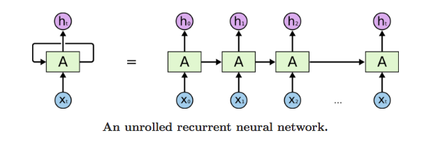
Recurrent Neural Network could be a generalization form of feed forward neural network that has an interior memory. RNN is recurrent in nature because it performs a similar operate for each input of information whereas the output of this input depends on the past one computation. When producing the output, it’s traced and sent back to the recurrent network. For making a decision, it considers this input and also the output that it’s learned from the previous input.
Unlike feed forward neural networks, RNNs will use their internal state (memory) to method sequences of inputs. This makes them applicable to tasks like united, connected handwriting recognition or speech recognition. In alternative neural networks, all the inputs are independent of every alternative. But in RNN, all the inputs are associated with one another.

First, it takes the X(0) from the sequence of input and so it outputs h(0) that along with X(1) is that the input for succeeding step. So, the h(0) and X(1) is that the input for succeeding step. Similarly, h(1) from succeeding is that the input with X(2) for succeeding step and then on. This way, it keeps basic cognitive process the context whereas training. The formula for the current state is

Applying Activation Function:

W is weight, h is that the single hidden vector, Whh is that the weight at previous hidden state, Whx is that the weight at current input state, tanh is that the Activation function, that implements a Non-linearity that squashes the activations to the range[-1,1].
Output:

Advantages of Recurrent Neural Networks:
1. RNN will model sequence of information in order that every sample is assumed to be captivated with previous ones.
2. Recurrent neural network are even used with convolutional layers to increase the effective picture element neighborhood.
Disadvantages of Recurrent Neural Networks:
1. Gradient vanishing and exploding issues.
2. Training an RNN could be a terribly tough task.
3. It cannot method terribly long sequences if using tanh or relu as an activation operate.
Applications of Recurrent Neural Networks:
1. Image Captioning
2. Generating poems
3. Reading Hand Writings
4. Music Generation
What is Long Short Term Memory (LSTM)?
Before diving into the LSTM, we should know about Vanishing Gradient and Exploding gradient problems.
Exploding and Vanishing Gradients:
During the training method of a network, the most goal is to reduce loss (in terms of error or cost) determined within the output once training data is distributed through it. We have a tendency to calculate the gradient, that is, loss with relation to a specific set of weights, modify the weights consequently and repeat this method till we get an best set of weights that loss is minimum. This is often the idea of backtracking. Sometimes, it thus happens that the gradient is sort of negligible. It should be noted that the gradient of a layer depends on certain parts within the sequential layers. If a number of these parts are tiny (less than 1), the result obtained, that is the gradient, are going to be even smaller. This is often referred to as the scaling impact. Once this gradient is increased with the training rate that is in itself a tiny low value ranging between 0.1–0.001, it ends up in a smaller value. As a consequence, the alteration in weights is kind of tiny, producing nearly an equivalent output as before. Similarly, if the gradients are quite massive in value because of the massive values of parts, the weights get updated to a value on the far side the best value. This is often referred to as the matter of exploding gradients. To avoid this scaling impact, the neural network unit was re-built in such how that the scaling issue was mounted to at least one. The cell was then enriched by many gating units and was referred to as LSTM.
Long short-term memory (LSTM) networks are a changed version of recurrent neural networks, that makes it easier to recollect past data in memory. The vanishing gradient downside of RNN is resolved. LSTM is well-suited to classify, method and predict time series given time lags of unknown length. It trains the model by using back-propagation.
In an LSTM network, 3 gates are present:

Input Gate : It would discover that value from input ought to be used to modify the memory. Sigmoid function decides which values to let through 0,1 and tanh function provides weightage to the values that are passed deciding their level of importance travel from-1 to 1.

Forget Gate : It would discover what details to be discarded from the block. It’s determined by the sigmoid function. It’s at the previous state(ht-1) and also the content input(Xt) and outputs a number between 0(omit this)and 1(keep this) for every number within the cell state Ct−1.

Output Gate : The input and also the memory of the block is employed to come to a decision the output. Sigmoid function decides that values to let through 0,1 and tanh function provides weightage to the values that are passed deciding their level of importance travel from-1 to 1 and increased with output of Sigmoid.

Drawbacks:
1. LSTMs became common as a result of they may solve the matter of vanishing gradients. However it seems, they fail to get rid of it fully. The matter lies within the undeniable fact that the information still should move from cell to cell for its analysis. Moreover, the cell has become quite advanced currently with the extra options (such as forget gates) being brought into the image.
2. They need a great deal of resources and time to urge trained and become prepared for real-world applications. In technical terms, they have high memory-bandwidth owing to linear layers present in every cell that the system typically fails to supply for. Thus, hardware-wise, LSTMs become quite inefficient.
3. With the increase of information mining, developers are trying to find a model which will keep in mind past data for a extended time than LSTMs. The supply of inspiration for such reasonably model is that the human habit of dividing a given piece of information into little components for straightforward remembrance.
4. LSTMs get tormented by completely different random weight initializations and therefore behave quite almost like that of a feed-forward neural internet. They like little weight initializations instead.
5. LSTMs are at risk of overfitting and it’s troublesome to use the dropout algorithmic rule to curb this issue. Dropout may be a regularization technique wherever input and recurrent connections to LSTM units are probabilistically excluded from activation and weight updates whereas training a network.
What is Sequence to Sequence Modelling ?
In a layman terms, if the input is passed into RNN/LSTM/GRU sequentially and generates outputs sequentially, then the modelling is called sequence to sequence modelling. Both input and output are sequences like Text, Numbers, Audio.

Why do we need Sequence to sequence modelling( Encoder-Decoder pair)?
RNN and LSTM alone cant be used for language generation or translation because there is no notion of synchrony between input and output and different languages have different grammar.
To map associate input sequence to associate output sequence, we frequently apply sequence-to-sequence transformation using associate encoder-decoder model. One example is that the use of seq2seq to translate a sentence from one language to a different.

Initially, the seq2seq model uses RNN, LSTM, or GRU to analyze the input sequence and to get the output sequence.
But this approach suffers a couple of setbacks.
Learning the long-range context with RNN gets tougher because the distance will increase.
To perceive the context of the word “view” below, we should always examine all the words during a paragraph at the same time i.e. to grasp what the “view” below could see, we should always apply fully-connected (FC) layers on to all the words within the paragraph.

However, this drawback involves high-dimensional vectors and makes it like finding a needle during a rick. But how the humans solve this problem? The solution could land on “attention”.
Attention Models:
Event the image below contains regarding 1M pixels, most of our attention could fall on the girl throwing a Frisbee.

When making a context for our question, we should always not place equal weight on all the information we get. We’d like to focus! We should always produce a context of what interests us based on the query. However this query can shift in time. For instance, if we are sorting out the Frisbee, our attention could focus within the air instead. Therefore how will we tend to create mentally this into equations and deep networks?

As like traditional RNN and LSTMs, input y are going to be replaced by the attention in associate attention-based system.

For example, for every input feature yᵢ, we will train associate FC layer to score how much important feature i is (or the pixel) underneath the context of the previous hidden state C.
Afterward, we tend to normalize the score employing a SoftMax perform to create the attention weights s.
Finally, the attention Z in substitution the input x are going to be the weighted output of the input features supported attention. Let’s develop the conception further before we tend to introduce the equations.
Query, Keys, Values (Q, K, V):
First, we are going to formalize the conception of attention with query, key, and value. Therefore what are query, key, and value? A query is that the context of what we tend to are trying to find. In previous equations, we tend to use the previous hidden state as the query context. We wish to grasp what’s next based on what we all know already. However in looking, it will merely a word provided by a user. Value is that the input features or raw pixels. Key’s merely associate encoded illustration for “value”. However in some cases, the “value” itself may be used as a “key”.


To create attention, we tend to confirm the connection between the query and therefore the keys. Then we tend to mask out the associated values that aren’t relevant to the query. For instance, for the query “girl”, the attention ought to specialize in the air and therefore the Frisbee.
Now, let’s see how we tend to apply attention to NLP and begin our transformer discussion. However the transformer is pretty complicated. It’s a completely unique encoder-decoder model attentively. It’ll take a while to debate it.
Transformers:
Many DL issues represent an input with a dense representation. This forces the model to extract vital information concerning the input. These extracted features are usually known as latent features, hidden variables, or a vector representation. Word embedding creates a vector illustration of a word that we are able to manipulate with algebra. However, a word will have totally different meanings in numerous contexts. Within the example below, word embedding uses constant vector in representing “bank” although they need totally different meanings within the sentence.
To create a dense representation of this sentence, we are able to take apart the sentence with an RNN to create an embedding vector. During this method, we have a tendency to bit by bit accumulate information in every timestep. However one could argue that once the sentence is obtaining longer, early info could also be forgotten or override.
Maybe, we should always convert a sentence to a sequence of vectors instead, i.e. one vector per word. Additionally, the context of a word are going to be considered throughout the encoding method. As an example, the word “bank” below are going to be treated and encoded otherwise in line with the context.

Let’s integrate this idea attentively using query, key, and value. We tend to decompose a sentence into single words. Every word acts as a value but conjointly as its key.

To encode the full sentence, we have a tendency to perform a query on every word. Thus a 21-word sentence ends up in twenty one queries and 21 vectors. This 21-vector sequence can represent the sentence.
So, how could we inscribe the sixteenth word “bank”? We have a tendency to use the word itself (“bank”) because the query. We reckon the connexons of this query with every key within the sentence. The representation of this word is solely a weighted add of the values per the relevance — the attention output. Conceptually, we tend to “grey out” non-relevant values to create the attention.

By browsing through Q₂₁, we tend to generate a twenty one attention (vector) sequence that represents the sentence.

Encoder part:
In the encoding step, the transformer uses learned word embedding to convert these thirteen words into thirteen 512-D word embedding vectors. Then they’re passed into an attention-based encoder to come up with the context-sensitive illustration for every word. Every word-embedding can have one output vector hᵢ, within the model usually we designed here, hᵢ could be a 512-D vector. It encodes the word xᵢ with its context.

Let’s zoom into this attention-based encoder a lot of. The encoder really stacks up 6 encoders with every encoder shown below. The output of an encoder is fed to the encoder higher than. This instance takes thirteen 512-D vectors and output thirteen 512-D vectors. For the primary decoder (encoder₁), the input is that the thirteen 512-D word embedding vectors.

Scaled Dot-Product Attention:
In every encoder, we need to perform attention initial. In our example, we’ve thirteen words and so thirteen queries. However we have a tendency to don’t reckon their attention on an individual basis.

Instead, all thirteen attentions is computed at the same time. We have a tendency to pack the queries, keys, and values into the matrix letter, K, and V severally. Every matrix can have a dimension of 13 × 512 (d=512). The matrix product QKᵀ can measure the similarity among the queries and also the keys.
However, once the dimension d is giant, we are going to encounter a problem with the dot products as said. Assume every row (q and k) in these matrices contains independent random variables with mean zero and variance one. Then their dot product q • k can have a mean zero and variance d (512). This can push a number of the dot product values to be terribly giant. This will move the SoftMax output to a low level gradient zone that needs an oversized modification within the dot product to form an apparent modification within the SoftMax output. This hurts the training progress. To correct that, the transformer divides the dot product with a multiplier factor equals to the root of the dimension.
Multi-Head Attention :
Multi-Head Attention generates h attentions per query. Conceptually, we have a tendency to simply pack h scaled dot-product attention along.

In the transformer, we have a tendency to use eight attentions per question. thus why can we want eight but not one attention as every attention will cover multiple areas anyway? Within the transformer, we don’t feed Q, K, and V on to the attention module. We tend to rework Q, K, and V severally with trainable matrix Wq, Wk, Wv first.

If we tend to use eight attentions, we are going to have eight totally different sets of projections higher than. This offers us eight totally different “perspectives”. This eventually pushes the accuracy higher, a minimum of through empirical observation. But, we would like to stay the computation quality similar. Thus rather than having the remodeled Q to own a dimension of 13 × 512, we need to scale it right down to 13 × 64. But now, we’ve eight attentions and eight reworked Qs.

The output is that the concatenate of the results from all the Scaled Dot-Product Attentions. Finally, we shall apply a linear transformation to the concatenated result with W. Note, we should describe the model as eight separate heads but within the coding, we pack all eight heads into a multi-dimensional Tensor and manipulate them as one unit.
Skip connection & Layer normalization:
This is the encoder using multi-head attention.

As shown, the transformer applies skip connection (residual blocks in ResNet) to the output of the multi-head attention followed by a layer normalization. each techniques create training easier and a lot of stable. In batch normalization, we have a tendency to normalize an output supported suggests that and variances collected from the training batches. In layer normalization, we use values within the same layer to perform the normalization instead. we’ll not elaborate on them more and it’s not vital to understanding them to find out the transformer. It’s simply a standard technique to form training a lot of stable and easier.
Position-wise Feed-Forward Networks:
Next, we would apply a fully-connected layer (FC), a ReLU activation, and another FC layer to the attention results. This operation is applied to every position individually and identically (sharing identical weights). It’s a position-wise feed-forward as a result of the ith output depends on the ith attention of the attention layer solely.

Similar to the attention, the transformer additionally uses skip connection and layer normalization.
Positional Encoding:

Convolution layers use restricted size filters to extract native info. So, for the primary sentence, “nice” can go together with “for you” rather than “requests”. Still, the transformer encodes a word with all its context quickly. Within the starting, “you” are going to be treated equally to “requests” in encoding the word “nice”. We tend to simply hope the model can extract and utilize the position and ordering info eventually. If failed, the inputs behave sort of a bag of words, and each sentences above can encode equally.
One attainable resolution is to produce position info as a part of the word embedding.

So, how will we tend to encode the position i into a 512-D input vector?
The equation below is employed for the fastened position embedding. This position embedding vector has 512 components, identical as the word embedding. The even components use the primary equation and also the odd components use the second equation to reckon the positional value. Once it’s comp we usually add the position embedding with the first word embedding to create the new word embedding.

This is the encoder. Next, we are going to discuss the decoder. Still, this section is facultative as a result of BERT uses the encoder solely.
BERT (Bidirectional Encoder Representations from Transformers)
With word embedding, we would produce a dense representation of words. However within the section of transformer, we will discover word embedding cannot explore the context of the neighboring words well. In NLI applications, we would like the model able to handle 2 sentences. Additionally, we would like a illustration model that’s multi-purposed. Natural language processing training is intense! Will we tend to pre-trained a model and repurpose it for alternative applications while not building a brand new model again?
Let’s have a fast outline of BERT. In BERT, a model is initial pre-trained with data that needs no human labeling. Once it’s done, the pre-trained model outputs a dense representation of the input. To resolve alternative natural language processing tasks, like QA, we would modify the model by merely adding a shallow DL layer connecting to the output of the initial model. Then, we have to retrain the model with information and labels specific to the task end-to-end.
In short, there’s a pre-training innovate that we would produce a dense illustration of the input (the left diagram below). The second part retunes the model with task-specific data, like MNLI or SQuAD, to resolve the target natural language processing downside.

Model:
BERT uses the transformer encoder we have mentioned to make the vector illustration.
Input / Output Representations:
But first, let’s outline how input is assembled and what output is predicted for the pre-trained model. First, the model must take one or 2 word-sequences to handle completely different spectrums of natural language processing tasks.

All input can begin with a special token [CLS] (a special classification token). If the input composes of 2 sequences, a [SEP] token can place between Sequence A and Sequence B.
If the input has T tokens, as well as the else tokens, the output can have T outputs additionally. Completely different elements of the output are going to be accustomed build predictions for various natural language processing tasks. The primary output is C (or typically written because the output [CLS] token). It’s the sole output used for any natural language processing classification task. For non-classification tasks with only 1 sequence, we can use the remaining outputs (without C).

So, how will we compose the input embedding? In BERT, the input embedding composes of word piece embedding, segment embeddings, and position embedding of an equivalent dimension. We could add them along to make the ultimate input embedding.

Instead of using each single word as tokens, BERT breaks a word into word items to scale back the vocabulary size (30,000 token vocabularies). As an example, the word “helping” is rotten into “help” and “ing”. Then it applies associate embedding matrix (V × H) to convert the one-hot vector Rⱽ for “help” to Rᴴ.
The segment embeddings model that sequence that tokens belong to. Will the token belong to the primary sentence or the second sentence? Thus it’s a vocabulary size of 2 (segment A or B). Intuitively, it adds a continuing offset to the embedding with value belonged to whether or not it belongs to sequence A or B. Mathematically, we can apply an embedding matrix (2 × H) to convert R² to Rᴴ. The last embedding is that the position embedding. It serves an equivalent purpose within the transformer in distinctive absolutely the or relative position of words.
Pretraining
BERT pre-trains the model with a pair of natural language processing tasks.
Masked LM
The first one is that the masked LM (Masked Language Model). We here use the transformer decoder to get a vector illustration of the input that some words masked.

Then BERT applies a shallow deep decoder to reconstruct the word sequence(s) back as well as the missing one.

In the masked Language Modeling, BERT masks out 15% of the WordPiece. 80% of the masked WordPiece are going to be replaced with a [MASK] token, 10% with a random token and 10% can keep the initial word. The loss is outlined as how well BERT predicts the missing word, not the reconstruction error of the entire sequence.

We don’t replace 100% of the missing WordPiece with the [MASK] token. This encourages the model to predict missing words, not the ultimate objective of making vector representations for the sequences with context taken into thought. BERT replaces 10% with random tokens and 10% with the initial words. This encourages the model to be told what could also be correct or what be wrong for the missing words.
Next Sentence Prediction (NSP):
The second pre-trained task is NSP. The key purpose is to make a representation within the output C which will encode the relations between Sequence A and B. To organize the training input, concerning 50% of the time, BERT uses 2 consecutive sentences as sequences A and B severally. BERT expects the model to predict “IsNext”, i.e. sequence B ought to follow sequence A. For the remaining 50% of the time, BERT selects two-word sequences arbitrarily and expect the prediction to be “Not Next”.

In this training, we can take the output C so classify it with a shallow classifier.

As noted, for each pre-training task, we can produce the training from a stiff with none human labeling.
These 2 coaching tasks facilitate BERT to train the vector illustration of 1 or 2 word-sequences. Aside from the context, it probably discovers alternative linguistics data as well as linguistics and grammatical relation.
Fine-tuning BERT:
Once the model is pre-trained, we will add a shallow classifier for any natural language processing task or a decoder, almost like what we could have mentioned within the pre-training step.

Then, we can work the task-related data and also the corresponding labels to refine all the model parameters end-to-end. That’s how the model is trained and refined. Thus BERT is a lot of on the training strategy instead of the model design. Its encoder is just the transformer encoder.
These are all about the core concepts of Natural Language Processing.
References:
POS, Lemmatizer, NLP, FE, DTM, NN, RNN, LSTM, ED
BERT: Pre-training of Deep Bidirectional Transformers for Language Understanding
